
RUBY
[CRIME] 11. seaborn 본문
서울시 범죄 현황 데이터 분석 프로젝트
11. seaborn
Seaborn은 Matplotlib을 기반으로 다양한 색상 테마와 통계용 차트 등의 기능을 추가한 시각화 패키지이다. 기본적인 시각화 기능은 Matplotlib 패키지에 의존하며 통계 기능은 Statsmodels 패키지에 의존한다.
1.
- seaborn은 matplotlib과 함께 실행된다.

!conda install -y seaborn
import numpy as np
import pandas as pd
import matplotlib.pyplot as plt
import seaborn as sns
from matplotlib import rc

plt.rcParams["axes.unicode_minus"] = False
rc("font", family="Malgun Gothic")
get_ipython().run_line_magic("matplotlib", "inline")
2.
- seaborn은 import하는 것만으로도 효과를 준다.
x = np.linspace(0, 14, 100)
y1 = np.sin(x)
y2 = 2 * np.sin(x + 0.5)
y3 = 3 * np.sin(x + 1.0)
y4 = 4 * np.sin(x + 1.5)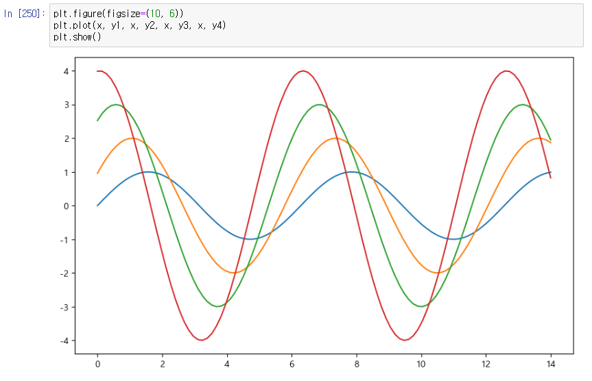
plt.figure(figsize=(10, 6))
plt.plot(x, y1, x, y2, x, y3, x, y4)
plt.show()
3. 스타일 주기
- sns.set_style()
- "white", "whitegrid", "dark", "darkgrid"
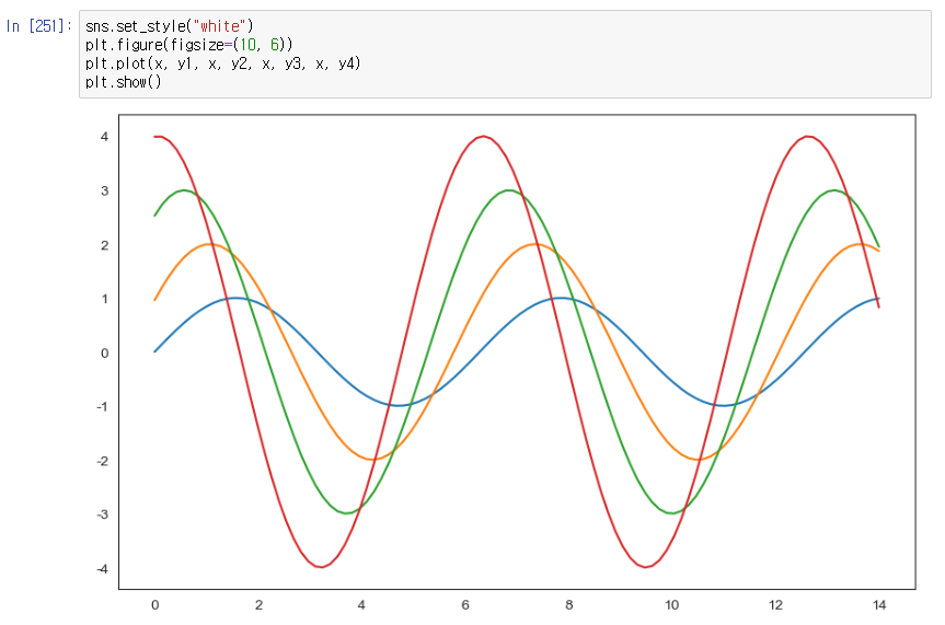
sns.set_style("white")
plt.figure(figsize=(10, 6))
plt.plot(x, y1, x, y2, x, y3, x, y4)
plt.show()
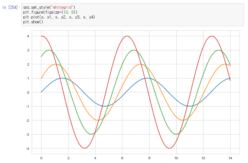
sns.set_style("whitegrid")
plt.figure(figsize=(10, 6))
plt.plot(x, y1, x, y2, x, y3, x, y4)
plt.show()
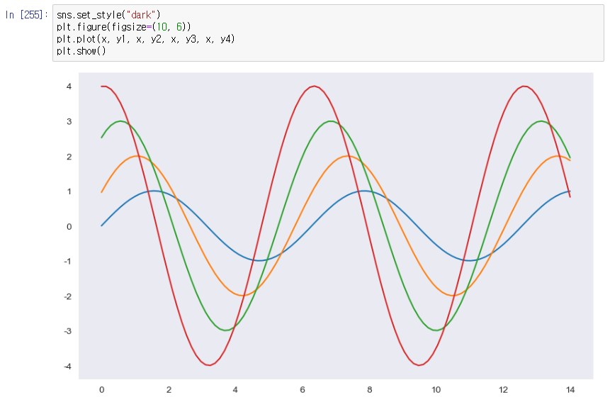
sns.set_style("dark")
plt.figure(figsize=(10, 6))
plt.plot(x, y1, x, y2, x, y3, x, y4)
plt.show()
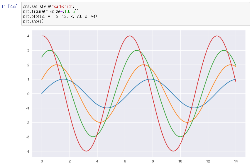
sns.set_style("darkgrid")
plt.figure(figsize=(10, 6))
plt.plot(x, y1, x, y2, x, y3, x, y4)
plt.show()
4.
- seaborn에는 실습용 데이터가 몇 개 내장되어 있다.
- 이 중 하나인 tips를 불러보자
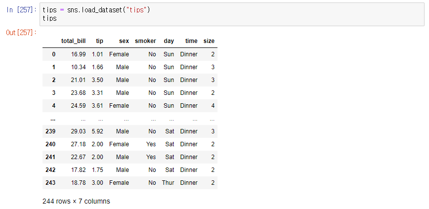
tips = sns.load_dataset("tips")
tips
5.
- tips의 정보 불러오기

tips.info()
6.
- boxplot을 그려볼 수 있다.
boxplot이란? 기술 통계학에서 '상자 수염 그림' 또는 '상자 그림'은 수치적 자료를 표현하는 그래프이다. 이 그래프는 가공하지 않은 자료 그대로를 이용하여 그린 것이 아니라, 자료로부터 얻어낸 통계량인 5가지 요약 수치를 가지고 그린다.
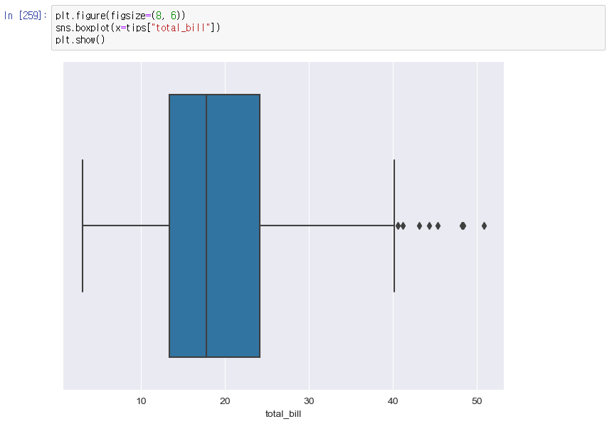
plt.figure(figsize=(8, 6))
sns.boxplot(x=tips["total_bill"])
plt.show()
7. boxplot에 컬럼을 지정하자.

tips["day"].unique()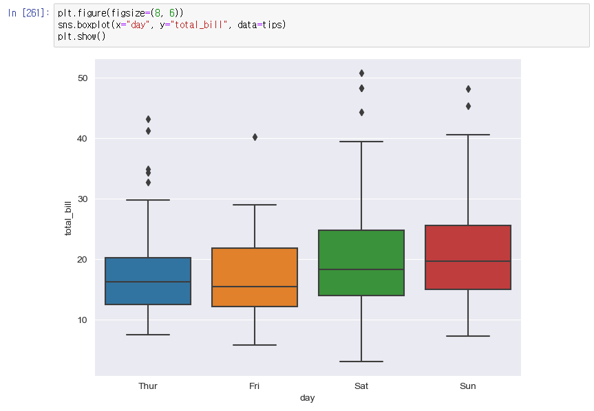
plt.figure(figsize=(8, 6))
sns.boxplot(x="day", y="total_bill", data=tips)
plt.show()
8. 칼럼을 지정하고 구분을 지을 수 있다.
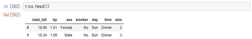
tips.head(2)
plt.figure(figsize=(8, 6))
sns.boxplot(x="day", y="total_bill", data=tips, hue="smoker", palette="Set1") # Set 1 ~ 3
plt.show()
9. swarmplot
- Strip plot과 violin plot의 조합이다.
- 데이터 포인트 수와 함께 각 데이터의 분포도 제공한다.
- Strip Plot에 비해 분포도를 확인하기 쉽다.
- color: 0~1 사이 검은색부터 흰색 사이 값을 조절
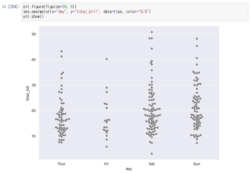
plt.figure(figsize=(8, 6))
sns.swarmplot(x="day", y="total_bill", data=tips, color="0.5")
plt.show()
10.
- boxplot을 swarmplot의 콜라보

plt.figure(figsize=(8, 6))
sns.boxplot(x="day", y="total_bill", data=tips)
sns.swarmplot(x="day", y="total_bill", data=tips, color="0.25")
plt.show()
11.
lmplot
- total bill과 tip 사이의 관계 파악
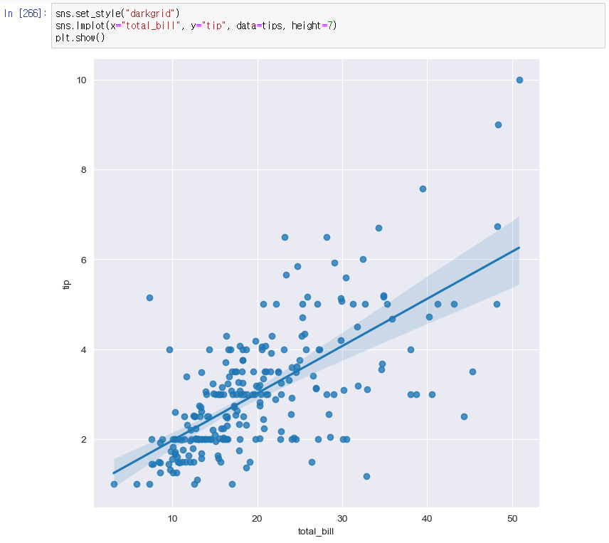
sns.set_style("darkgrid")
sns.lmplot(x="total_bill", y="tip", data=tips, height=7)
plt.show()
12.
- implot에서 hue옵션을 사용해보자
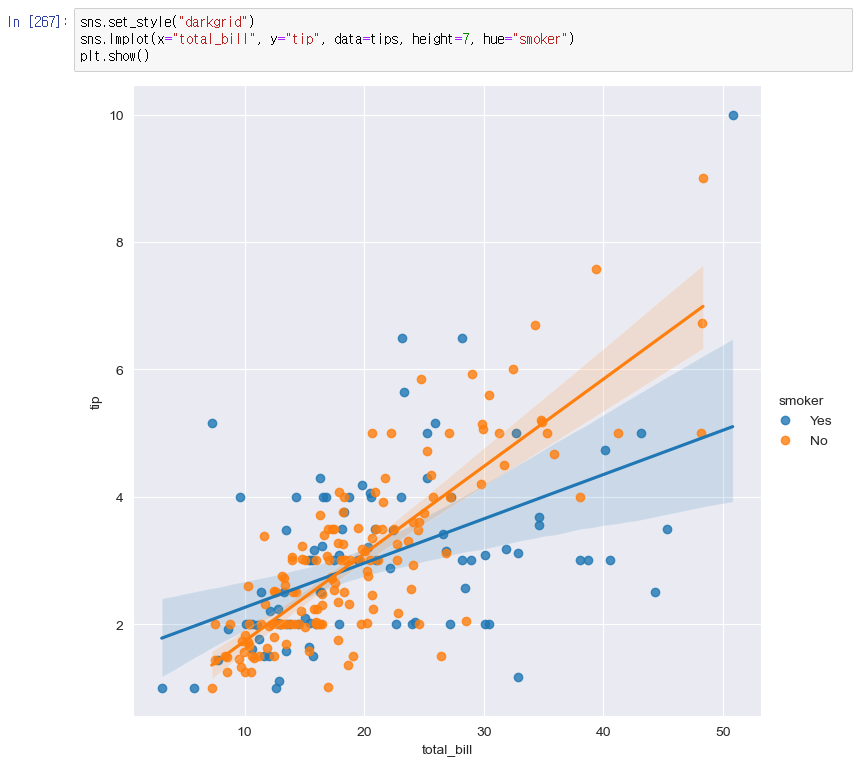
sns.set_style("darkgrid")
sns.lmplot(x="total_bill", y="tip", data=tips, height=7, hue="smoker")
plt.show()
13.
flights data(기본으로 담겨있는 데이터)
- heatmap
- heatmap은 열을 의미하는 heat와 지도를 뜻하는 map을 합친 단어이다. 데이터들의 배열을 색상으로 표현해주는 그래프이다.
- heatmap을 사용하면 두 개의 카테고리 값에 대한 값 변화를 한 눈에 알기 쉽다.
- 대용량 데이터도 heatmap을 이용해 시각화한다면 이미지 몇장으로 표현이 가능하다.
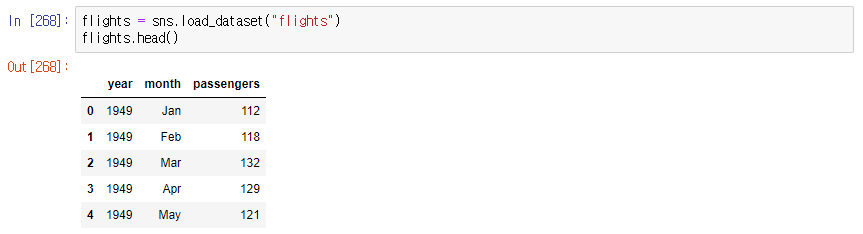
flights = sns.load_dataset("flights")
flights.head()
14. pivot 옵션을 사용할 수도 있다.

flights = flights.pivot(index="month", columns="year", values="passengers")
flights.head()
15. heatmap을 이용하면 전체 경향을 알 수 있다.
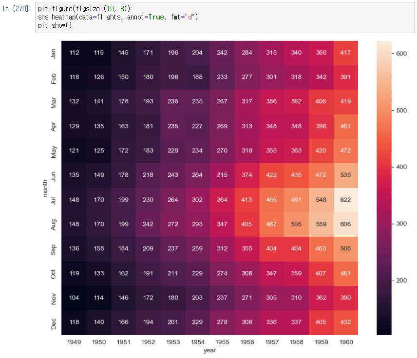
plt.figure(figsize=(10, 8))
sns.heatmap(data=flights, annot=True, fmt="d")
plt.show()
16. colormap을 조금 다르게 보자

plt.figure(figsize=(10, 8))
sns.heatmap(flights, annot=True, fmt="d", cmap="YlGnBu")
plt.show()
17. iris data
- pairplot
데이터에 들어 있는 각 컬럼(열)들의 모든 상관 관계를 출력
3차원 이상의 데이터라면 pairplot 함수를 사용해 분포도를 그립니다.
pairplot은 그리도(grid) 형태로 각 집합의 조합에 대해 히스토그램과 분포도를 그립니다.
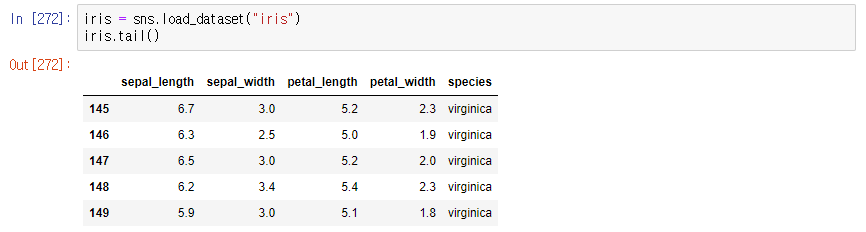
iris = sns.load_dataset("iris")
iris.tail()
18. 다수의 컬럼을 비교하는 pairplot
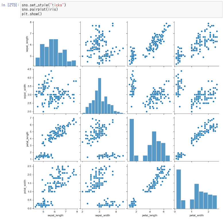
sns.set_style("ticks")
sns.pairplot(iris)
plt.show()
pairplot에서도 hue 옵션을 사용해보자
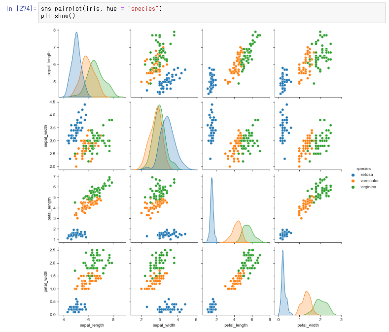
sns.pairplot(iris, hue = "species")
plt.show()
19. 원하는 컬럼만 pairplot
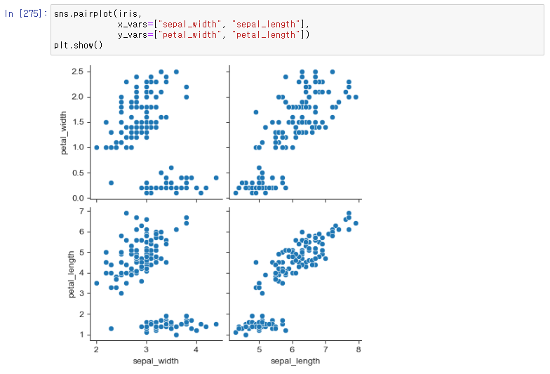
sns.pairplot(iris,
             x_vars=["sepal_width", "sepal_length"],
             y_vars=["petal_width", "petal_length"])
plt.show()
20. anscombe 데이터를 가져와보자
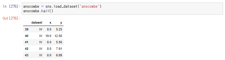
anscombe = sns.load_dataset("anscombe")
anscombe.tail()
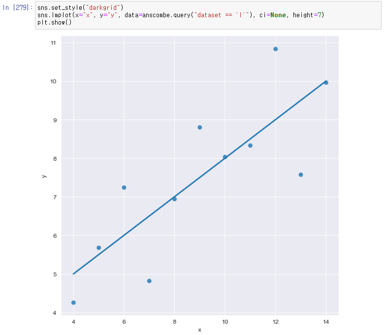
sns.set_style("darkgrid")
sns.lmplot(x="x", y="y", data=anscombe.query("dataset == 'I'"), ci=None, height=7)
plt.show()
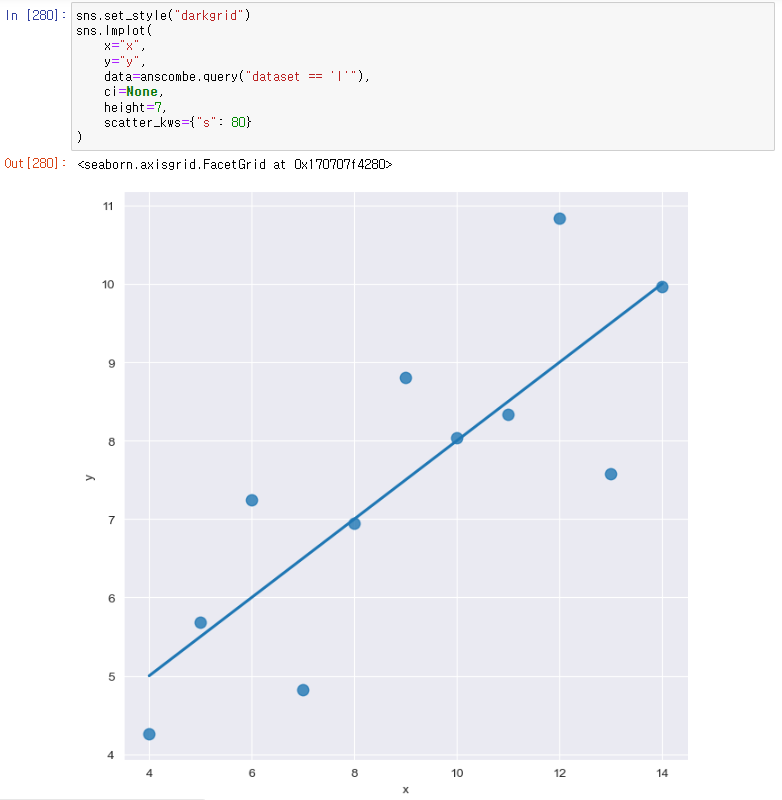
sns.set_style("darkgrid")
sns.lmplot(
    x="x",
    y="y",
    data=anscombe.query("dataset == 'I'"),
    ci=None,
    height=7,
    scatter_kws={"s": 80}
)
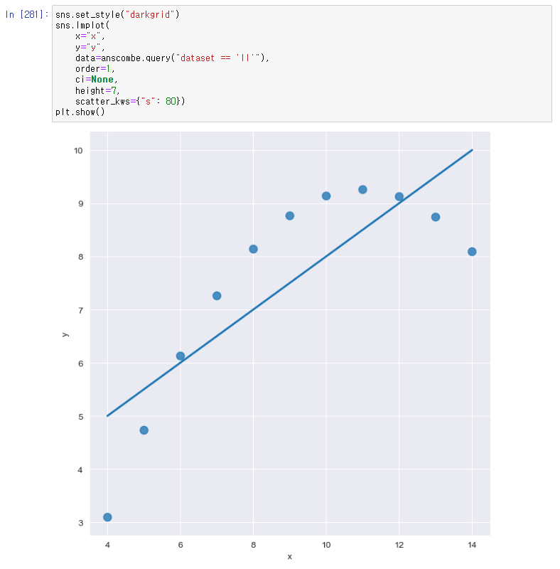
sns.set_style("darkgrid")
sns.lmplot(
    x="x",
    y="y",
    data=anscombe.query("dataset == 'II'"),
    order=1,
    ci=None,
    height=7,
    scatter_kws={"s": 80})
plt.show()
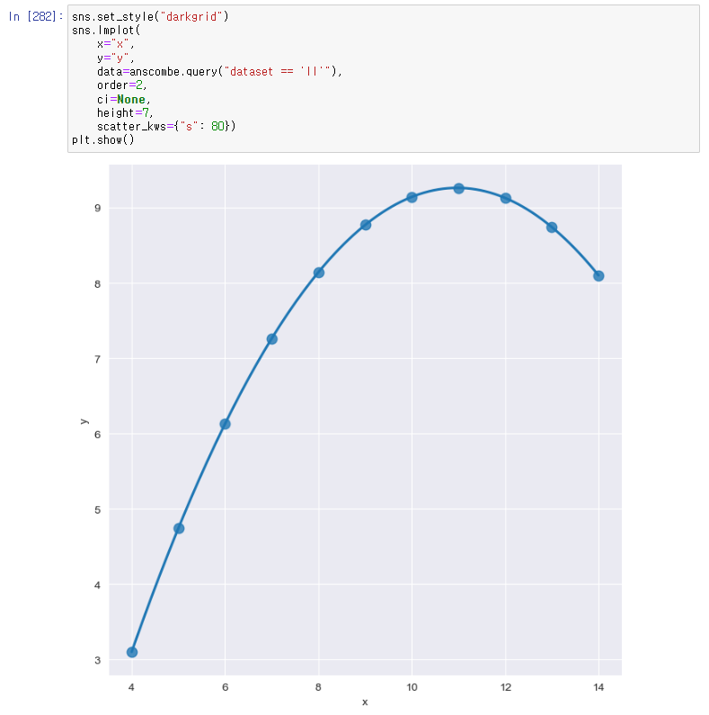
sns.set_style("darkgrid")
sns.lmplot(
    x="x",
    y="y",
    data=anscombe.query("dataset == 'II'"),
    order=2,
    ci=None,
    height=7,
    scatter_kws={"s": 80})
plt.show()
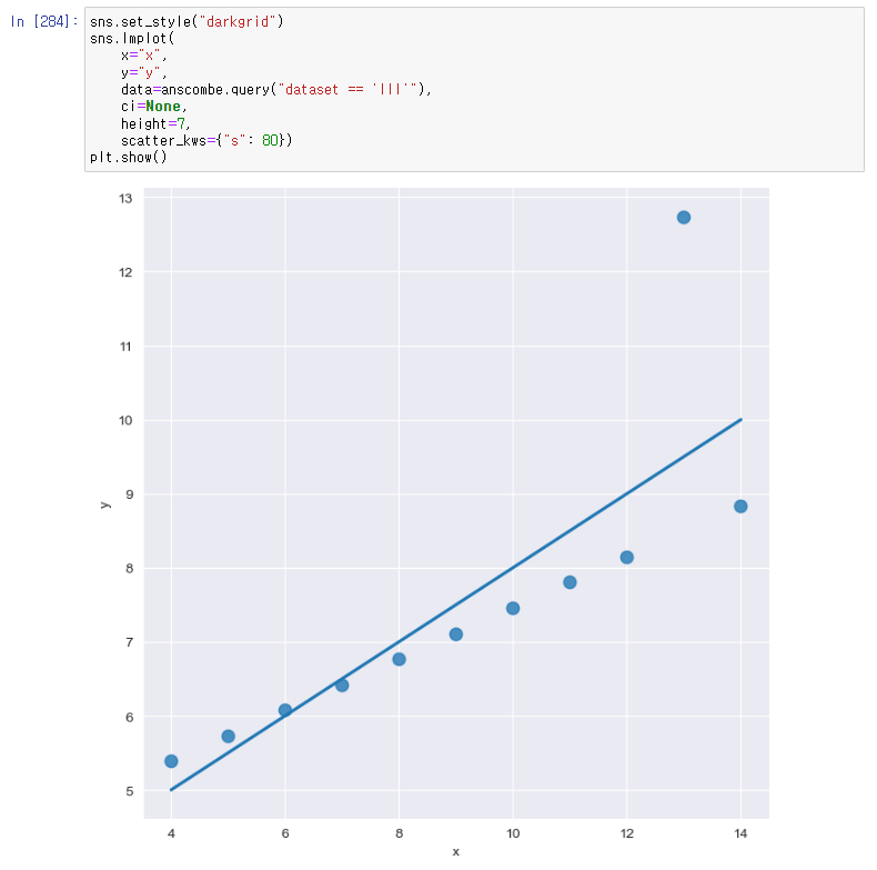
sns.set_style("darkgrid")
sns.lmplot(
    x="x",
    y="y",
    data=anscombe.query("dataset == 'III'"),
    ci=None,
    height=7,
    scatter_kws={"s": 80})
plt.show()
'데이터 분석 > EDA_웹크롤링_파이썬프로그래밍' 카테고리의 다른 글
| [CRIME] 13. 지도 시각화(Folium) (0) | 2023.02.04 |
|---|---|
| [CRIME] 12. 서울시 범죄현황 데이터 시각화(pair plot, heat map) (0) | 2023.02.03 |
| [CRIME] 10. 범죄 데이터 정렬을 위한 데이터 정리 (0) | 2023.02.03 |
| [CRIME] 9. 구별 데이터 얻기 (1) | 2023.02.03 |
| [CRIME] 8. Google Maps을 이용한 데이터 정리 (1) | 2023.02.03 |


